Sorting is a basic building block that many other algorithms are built upon. It’s related to several exciting ideas that you’ll see throughout your programming career. Understanding how sorting algorithms work behind the scenes is a fundamental step toward implementing correct and efficient algorithms that solve real-world problems.

• How different sorting algorithms work and how they compare under different circumstances

• How built-in sort functionality works behind the scenes

• How different computer science concepts like recursion and divide and conquer apply to sorting

• How to measure the efficiency of an algorithm using Big O notation

You’ll understand sorting algorithms from both a theoretical and a practical standpoint. More importantly, you’ll have a deeper understanding of algorithm design techniques that you can apply to other work areas. Let’s get started!

The Importance of Sorting Algorithms in Python

Sorting is one of the most thoroughly studied algorithms in computer science. There are dozens of different sorting implementations and applications that you can use to make your code more efficient and effective.

You can use sorting to solve a wide range of problems:

• Searching: Searching for an item on a list works much faster if the list is sorted.

• Selection: Selecting items from a list based on their relationship to the rest of the items is easier with sorted data. For example, finding the kth-largest or smallest value, or finding the median value of the list, is much easier when the values are in ascending or descending order.

• Duplicates: Finding duplicate values on a list can be done very quickly when the list is sorted.

• Distribution: Analyzing the frequency distribution of items on a list is very fast if the list is sorted. For example, finding the element that appears most or least often is relatively straightforward with a sorted list.

Since they can often reduce the complexity of a problem. These algorithms have direct applications in searching algorithms, database algorithms, divide and conquer methods, data structure algorithms, and many more.

From commercial applications to academic research and everywhere in between, there are countless ways you can use sorting to save yourself time and effort.

Trade-Offs of Sorting Algorithms

When choosing a sorting algorithm, some questions have to be asked – How big is the collection being sorted? How much memory is available? Does the collection need to grow?

The answers to these questions may determine which algorithm is going to work best for each situation. Some algorithms like merge sort may need a lot of space or memory to run, while insertion sort is not always the fastest, but doesn't require many resources to run.

You should determine what your requirements are, and consider the limitations of your system before deciding which sorting algorithm to use.

Some Common Sorting Algorithms

Some of the most common sorting algorithms are:

• Selection sort

• Bubble sort

• Insertion sort

• Merge sort

• Quick sort

• Heap sort

• Counting sort

• Radix sort

• Bucket sort

But before we get into each of these, let's learn a bit more about what classifies a sorting algorithm.

Classification of a Sorting Algorithm

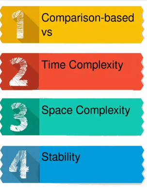
Sorting algorithms can be categorized based on the following parameters:

1. The number of swaps or inversions required: This is the number of times the algorithm swaps elements to sort the input. Selection sort requires the minimum number of swaps.

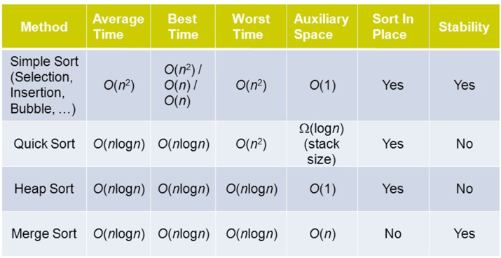
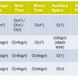
2. The number of comparisons: This is the number of times the algorithm compares elements to sort the input. Using Big-O notation, the sorting algorithm examples listed above require at least O(nlogn) comparisons in the best case, and O(n^2) comparisons in the worst case for most of the outputs.

3. Whether or not they use recursion: Some sorting algorithms, such as quick sort, use recursive techniques to sort the input. Other sorting algorithms, such as selection sort or insertion sort, use non-recursive techniques. Finally, some sorting algorithms, such as merge sort, make use of both recursive as well as non-recursive techniques to sort the input.

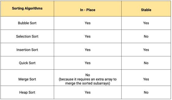
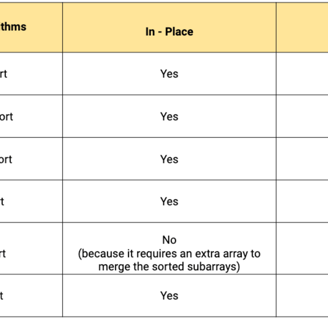
4. Whether they are stable or unstable: Stable sorting algorithms maintain the relative order of elements with equal values, or keys. Unstable sorting algorithms do not maintain the relative order of elements with equal values / keys.

For example, imagine you have the input array [1, 2, 3, 2, 4]. And to help differentiate between the two equal values, 2, let's update them to 2a and 2b, making the input array [1, 2a, 3, 2b, 4].

Stable sorting algorithms will maintain the order of 2a and 2b, meaning the output array will be [1, 2a, 2b, 3, 4]. Unstable sorting algorithms do not maintain the order of equal values, and the output array may be [1, 2b, 2a, 3, 4].

Insertion sort, merge sort, and bubble sort are stable. Heap sort and quick sort are unstable.

5. The amount of extra space required: Some sorting algorithms can sort a list without creating an entirely new list. These are known as in-place sorting algorithms, and require a constant O(1) extra space for sorting. Meanwhile, out of place sorting algorithms create a new list while sorting.

Insertion sort and quick sort are in place sorting algorithms, as elements are moved around a pivot point, and do not use a separate array.

Merge sort is an example of an out of place sorting algorithm, as the size of the input must be allocated beforehand to store the output during the sort process, which requires extra memory.

Sorting happens CONSTANTLY, and actually represents a huge portion of all computer and internet activity. Each with different approaches to get to the same or similar results.

But which one is best if they (almost) all return the same result?

Best usually means which is fastest. This is where “Big O” came into play.

Big O notation, sometimes also called “asymptotic analysis”, primarily looks at how many operations a sorting algorithm takes to completely sort a very large collection of data. This is a measure of efficiency and is how you can directly compare one algorithm to another.

When building a simple app with only a few pieces of data to work through, this sort of analysis is unnecessary. But when working with very large amounts of data, like a social media site or a large e-commerce site with many customers and products, small differences between algorithms can be significant.

The Significance of Time Complexity

The two different ways to measure the runtime of sorting algorithms:

1. For a practical point of view, you’ll measure the runtime of the implementations using the timeit module.

2. For a more theoretical perspective, you’ll measure the runtime complexity of the algorithms using Big O notation.

Measuring Efficiency With Big O Notation

The specific time an algorithm takes to run isn’t enough information to get the full picture of its time complexity. To solve this problem, you can use Big O (pronounced “big oh”) notation. Big O is often used to compare different implementations and decide which one is the most efficient, skipping unnecessary details and focusing on what’s most important in the runtime of an algorithm.(as we seen above)

The time in seconds required to run different algorithms can be influenced by several unrelated factors, including processor speed or available memory. Big O, on the other hand, provides a platform to express runtime complexity in hardware-agnostic terms. With Big O, you express complexity in terms of how quickly your algorithm’s runtime grows relative to the size of the input, especially as the input grows arbitrarily large.

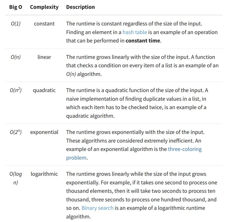
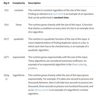
Assuming that n is the size of the input to an algorithm, the Big O notation represents the relationship between n and the number of steps the algorithm takes to find a solution. Big O uses a capital letter “O” followed by this relationship inside parentheses. For example, O(n) represents algorithms that execute a number of steps proportional to the size of their input.

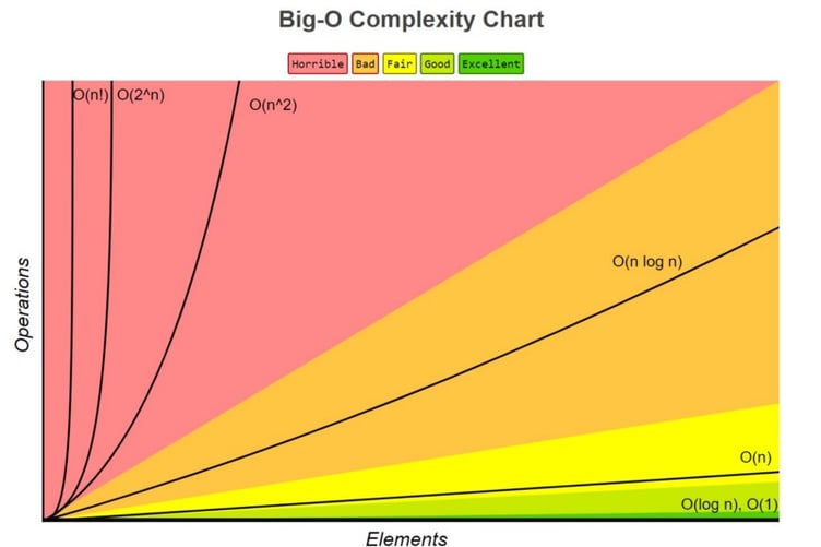
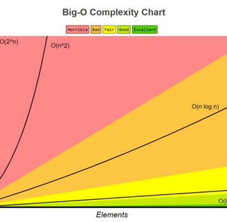
Here are five examples of the runtime complexity of different algorithms

Big O notation ranks an algorithms’ efficiency

It does this with regard to “O” and “n”, ( example: “O(log n)” ), where

• O refers to the order of the function, or its growth rate, and

• n is the length of the array to be sorted.

Let’s work through an example. If an algorithm has the number of operations required formula of:

f (n) = 6n^4 - 2n^3 + 5

As “n” approaches infinity (for very large sets of data), of the three terms present, 6n^4 is the only one that matters. So the lesser terms, 2n^3 and 5, are actually just omitted because they are insignificant. Same goes for the “6” in 6n^4, actually.

Therefore, this function would have an order growth rate, or a “big O” rating, of O(n^4) .

When looking at many of the most commonly used sorting algorithms, the rating of O(n log n) in general is the best that can be achieved. Algorithms that run at this rating include Quick Sort, Heap Sort, and Merge Sort. Quick Sort is the standard and is used as the default in almost all software languages.

When looking at many of the most commonly used sorting algorithms, the rating of O(n log n) in general is the best that can be achieved. Algorithms that run at this rating include Quick Sort, Heap Sort, and Merge Sort. Quick Sort is the standard and is used as the default in almost all software languages.

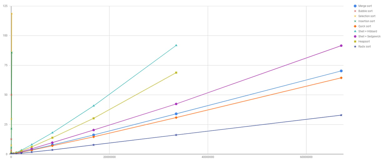
As you can see from the image, RadixSort is generally the fastest, followed by QuickSort. Their time complexities are:

• RadixSort: O(N*W), where N is the number of elements to sort and W is the number of bits required to store each key.

• QuickSort: O(N*logN), where N is the number of elements to sort.

Anyway, RadixSort speed comes at a cost. In fact, the space complexities of the two algorithms are the following:

• RadixSort: O(N+W), where N is the number of elements to sort and W is the number of bits required to store each key.

• QuickSort: O(logN), or O(N) depending on how the pivots are chosen.

Bucket Sort

Bucket sort is a comparison sort algorithm that operates on elements by dividing them into different buckets and then sorting these buckets individually. Each bucket is sorted individually using a separate sorting algorithm like insertion sort, or by applying the bucket sort algorithm recursively.

Bucket sort is mainly useful when the input is uniformly distributed over a range. For example, imagine you have a large array of floating point integers distributed uniformly between an upper and lower bound.

You could use another sorting algorithm like merge sort, heap sort, or quick sort. However, those algorithms guarantee a best case time complexity of O(nlogn).

Using bucket sort, sorting the same array can be completed in O(n) time.

Pseudo Code for Bucket Sort:

Counting Sort

The counting sort algorithm works by first creating a list of the counts or occurrences of each unique value in the list. It then creates a final sorted list based on the list of counts.

One important thing to remember is that counting sort can only be used when you know the range of possible values in the input beforehand.

Properties

• Space complexity: O(k)

• Best case performance: O(n+k)

• Average case performance: O(n+k)

• Worst case performance: O(n+k)

• Stable: Yes (k is the range of the elements in the array)

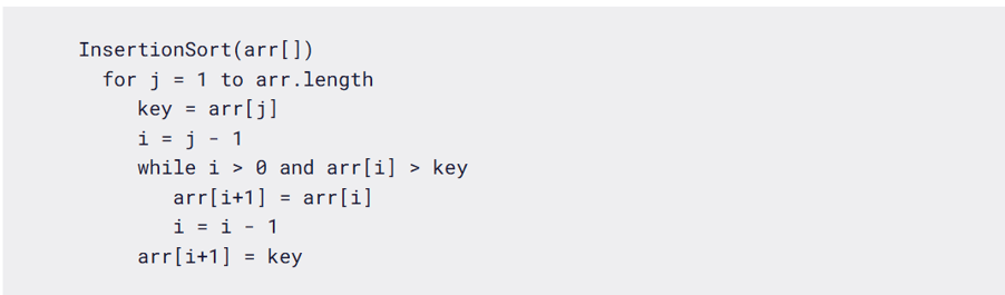
Insertion Sort

Insertion sort is a simple sorting algorithm for a small number of elements.

Example:

In Insertion sort, you compare the key element with the previous elements. If the previous elements are greater than the key element, then you move the previous element to the next position.

Start from index 1 to size of the input array.

[ 8 3 5 1 4 2 ] -> [1 2 3 4 5 8]

The algorithm shown below is a slightly optimized version to avoid swapping the key element in every iteration. Here, the key element will be swapped at the end of the iteration (step).

Properties:

• Space Complexity: O(1)

• Time Complexity: O(n), O(n n), O(n n) for Best, Average, Worst cases respectively.

• Best Case: array is already sorted

• Average Case: array is randomly sorted

• Worst Case: array is reversely sorted.

• Sorting In Place: Yes

• Stable: Yes

Heapsort

Heapsort is an efficient sorting algorithm based on the use of max/min heaps. A heap is a tree-based data structure that satisfies the heap property – that is for a max heap, the key of any node is less than or equal to the key of its parent (if it has a parent).

This property can be leveraged to access the maximum element in the heap in O(logn) time using the maxHeapify method. We perform this operation n times, each time moving the maximum element in the heap to the top of the heap and extracting it from the heap and into a sorted array. Thus, after n iterations we will have a sorted version of the input array.

The algorithm is not an in-place algorithm and would require a heap data structure to be constructed first. The algorithm is also unstable, which means when comparing objects with same key, the original ordering would not be preserved.

This algorithm runs in O(nlogn) time and O(1) additional space [O(n) including the space required to store the input data] since all operations are performed entirely in-place.

The best, worst and average case time complexity of Heapsort is O(nlogn). Although heapsort has a better worse-case complexity than quicksort, a well-implemented quicksort runs faster in practice. This is a comparison-based algorithm so it can be used for non-numerical data sets insofar as some relation (heap property) can be defined over the elements.

Properties:

• Space Complexity: O(1)

• Time Complexity: O(nlogn), O(nlogn), O(nlogn) for Best, Average, Worst cases respectively.

• Best Case: array is already sorted

• Average Case: array is randomly sorted

• Worst Case: array is reversely sorted.

• Sorting In Place: Yes

• Stable: No

Sorting Algorithms Explained with Examples in JavaScript, Python, Java, and C++